Make art with Stable Diffusion
An exploration of Stable Diffusion and its applications
Table of contents
Stable Diffusion is a collection of open-source models by Stability AI. They are used to generate images, most commonly as text to image models: you give it a text prompt, and it returns an image. But they can also be used for inpainting and outpainting, image-to-image (img2img) and a lot more.
In this guide we’ll show you the basics, then dive deeper into using these models to get the best out of them.
Try it first
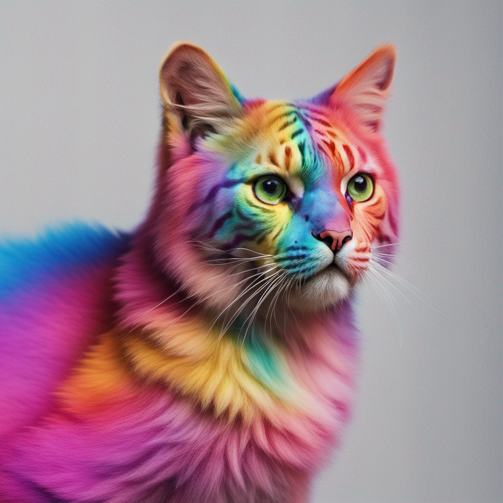
If you haven’t used Stable Diffusion before, give it a go now. Visit Stable Diffusion XL and try asking for a painting of a cute cat.
The text prompt is the only required input to generate an image using Stable Diffusion, but there are many other inputs like negative prompt, output image dimensions, and inference steps that can be used to control the output. When you run Stable Diffusion on Replicate, you can customize all of these inputs to get a more specific result.
The models
There are many different versions of Stable Diffusion. Let’s break it down:
- Stable Diffusion XL (SDXL) is currently the most popular version of Stable Diffusion. It was released in July 2023 and creates fantastic, realistic images around the 1024x1024 resolution, though you can use any aspect ratio.
- Stable Diffusion 1.5 (SD1.5) is an older version that was open-sourced in August 2022, and its images are best at 512x512. Despite its age, it remains popular because of its speed, low memory usage, and an abundance of community fine-tuned models which use SD1.5 as a base.
- Stable Diffusion 2.1 (SD2.1) was released in October 2022, and was “sort of like the awkward second album”. Good, just… different. This version introduced improvements like negative prompts, OpenCLIP for a text encoder, larger image outputs, but the migration to OpenClip caused significant changes to the image output and composition, when compared to prior versions of Stable Diffusion. To many, this felt like a “breaking change”. Most notably, this migration caused many artist’s names to be removed from the text encoder, which to this day drives a subset of users to use 1.5 or SDXL over version 2.
- SDXL Turbo is a version of SDXL that was released in November 2023. It is a non-commercial model that is very fast and can make good images in a single step.
- SD Turbo is another fast and non-commercial version that was released in November 2023.
Sections in this guide
- How to use Stable Diffusion
A guide to all the Stable Diffusion parameters - Image to image (img2img)
How to use an image as a reference - Inpainting
How to edit parts of an image - Outpainting
How to edit beyond the canvas of an existing image - Fine-tuning
Dreambooth, LoRAs, Textual Inversion and training with an API - Controlnet
An explanation of controlnets and their preprocessors - Turbo and LCMs
An explanation of very fast, few steps, Stable Diffusion - Glossary
An explanation of common Stable Diffusion terms
How to use Stable Diffusion
Let’s cover the basics. These are the parameters you’ll see when using Stable Diffusion:
- prompt
- negative prompt
- width and height
- steps (or number of inference steps)
- guidance scale (classifier-free guidance scale, or CFG scale)
- seed
- scheduler (or sampler)
- batch size
Prompt
The most important parameter is the prompt. It’s a text prompt that tells the model what image to generate.
Generally you should:
- use comma separated terms (do not prompt Stable Diffusion like you would talk to ChatGPT)
- put the most important thing first
- keep your prompt within 75 tokens (or about 60 words)
Example prompts:
- a photo of a cat, photography, studio portrait, 50mm lens
- an oil painting of a cat, abstract, impressionism, 1920s
Negative prompt
A negative prompt is a list of all the things you don’t want in your image. Write it in the same way you would a normal prompt: comma separated terms, with the most important thing first.
If you’re asking for a ‘photo of a cat’, and you’re getting back results that look like paintings or illustrations instead of a photo, put ‘painting, illustration’ in your negative prompt.
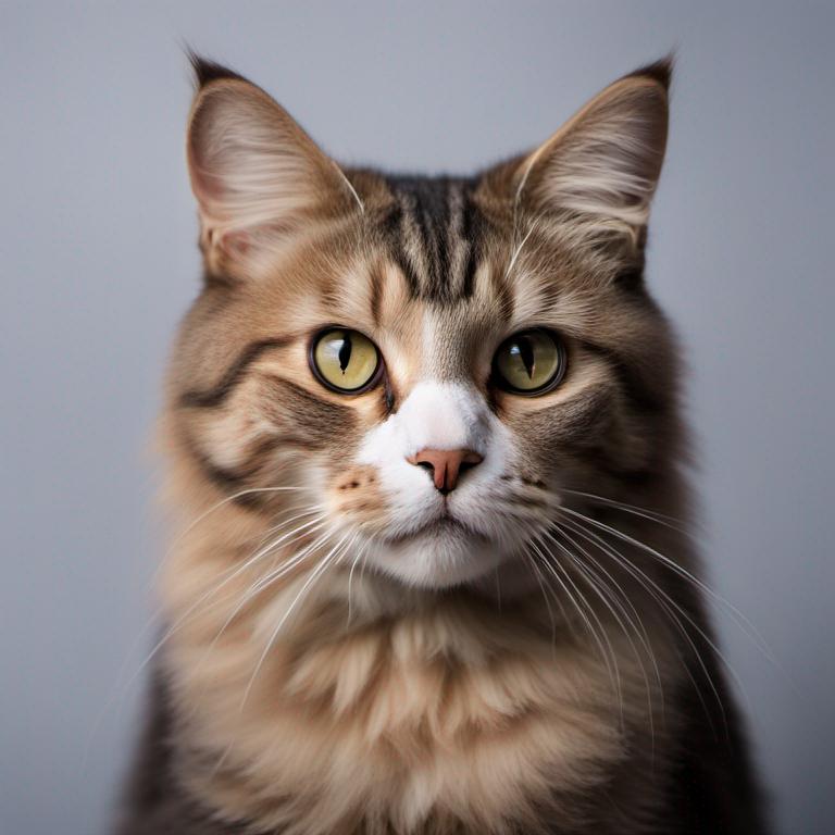
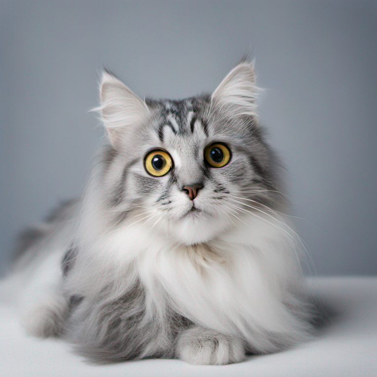
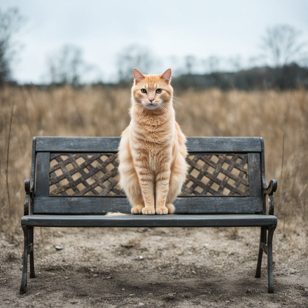
Let’s take our previous cat example and add a negative prompt to see the difference. Imagine that we didn’t want a brown cat, and we didn’t want a cat that looked so serious, so we’ll use the negative prompt: ‘brown cat, serious’:
Width and height
For Stable Diffusion 1.5, outputs are optimised around 512x512 pixels. Many common fine-tuned versions of SD1.5 are optimised around 768x768.
The best resolutions for common aspect ratios are typically:
- 1:1 (square): 512x512, 768x768
- 3:2 (landscape): 768x512
- 2:3 (portrait): 512x768
- 4:3 (landscape): 768x576
- 3:4 (portrait): 576x768
- 16:9 (widescreen): 912x512
- 9:16 (tall): 512x912
For SDXL, outputs are optimised around 1024x1024 pixels. The best resolutions for common aspect ratios are typically:
- 1:1 (square): 1024x1024, 768x768
- 3:2 (landscape): 1152x768
- 2:3 (portrait): 768x1152
- 4:3 (landscape): 1152x864
- 3:4 (portrait): 864x1152
- 16:9 (widescreen): 1360x768
- 9:16 (tall): 768x1360
Width and height must be divisible by 8.
If you want to generate images larger than this, we recommend using an upscaler.
View our collection of upscaling models.
Number of inference steps
This is the number of steps the model will take to generate your image.
A larger number of steps increases the quality of the output but it takes longer to generate.
For vanilla SDXL and Stable Diffusion 1.5 you should start with a value of about 20 steps. Don’t go too high though, because after a point each step helps less and less. 50 steps is a good maximum.
Recent models like SDXL Turbo and SD Turbo can generate high quality images in just a single step, making them exceptionally fast.
Seed
A seed is a number used to initialize randomness for the model. By setting a seed, you can get the same output every time.
If you find an image you like but want to tweak it or improve quality, you can use the same seed and change other parameters.
For example, keep the same seed and:
- increase the number of steps to improve quality
- tweak the prompt to tweak the image
- experiment with guidance scale
If you have a fixed seed but change the width or height of the image, then you will not see consistent results.
Guidance scale
The guidance scale tells the model how similar the output should be to the prompt. Start with a value of 7 or 7.5.
If your outputs aren’t matching your prompt as much as you’d like, try increasing this number. If you want the AI to be more creative, lower it.
SDXL Turbo and SD Turbo do not use a guidance scale. If the tool you use has an option for it, set it to 0.
Scheduler (or sampler)
Choosing a scheduler is an advanced parameter. They play a critical role in determining how the noise is incrementally reduced (denoising) to form the final output.
Many users will have a favorite scheduler and stick with it. Most schedulers give similar results, but some can sample faster, while others can get good results in fewer steps.
We recommend starting with Euler or Euler ancestral (EULER_A), a good scheduler for both SD1.5 and SDXL.
DPM++ 2M Karras is a popular choice among users of AUTOMATIC1111, which is a user interface tool for Stable Diffusion.
Batch size
This is the number of images that will be generated at once. A larger batch size needs more memory, but time per image is usually reduced.
The number of images you can batch at once is limited by the memory available.
On Replicate, SDXL image generation is limited to batches of 4.
Newer models that produce images in fewer steps also use less memory, and can batch more images at once.
Image to image (img2img) with Stable Diffusion
Use image-to-image to take the features and structure of a starting image and reimagine them with a prompt. The colors in your original image will be preserved.
Prompt strength (or denoising strength)
This only applies to image-to-image and inpainting generations.
It determines how much of your original image will be changed to match the given prompt.
Higher numbers change more of the image, lower numbers keep the original image intact. Values between 0.5 and 0.75 give a good balance.
When inpainting, setting the prompt strength to 1 will create a completely new output in the inpainted area.
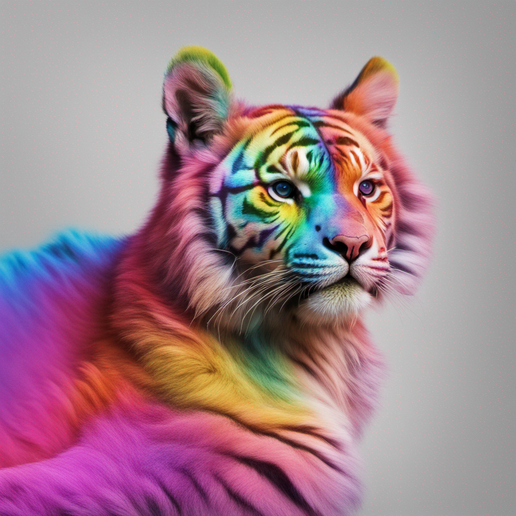
Using prompt strength 0.95
In this example we’ve increased the prompt strength. You can see that the image has changed a lot, it matches the prompt more closely and our original cat is very much a tiger.
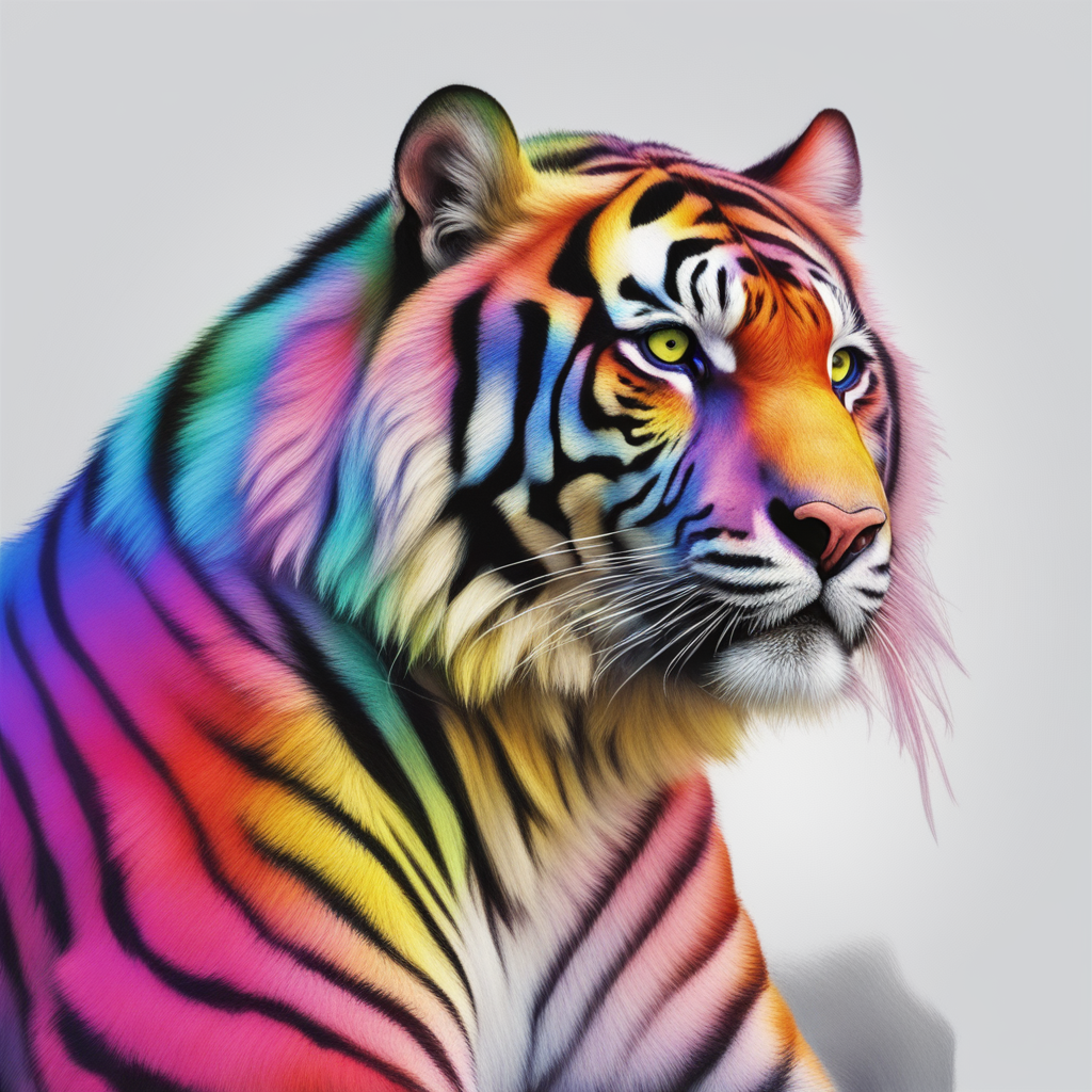
Using prompt strength 0.45
If we do the opposite, and reduce the prompt strength, you can see that much more of the original image is preserved. Our cat has only slightly changed, and it’s showing minor tiger-like features.
Inpainting with Stable Diffusion
Inpainting is like an AI-powered erasing and painting tool.
It can be used to:
- remove unwanted objects from an image
- replace or change existing objects in an image
- fix ugly or broken parts of a previously generated image
- expand the canvas of an image (outpainting)
It is similar to image-to-image.
Check out inpainter.app and outpainter.app to play around with interactive interfaces for inpainting and outpainting.
Prompt strength and inpainting
You can use the ‘prompt strength’ parameter to change how much the starting image guides the area being inpainted.
A value of 0.65 will keep the same colors and some of the structure that was there before, but will also generate new content based on the prompt.
Setting prompt strength to 1 will completely ignore the original image and only generate new content.
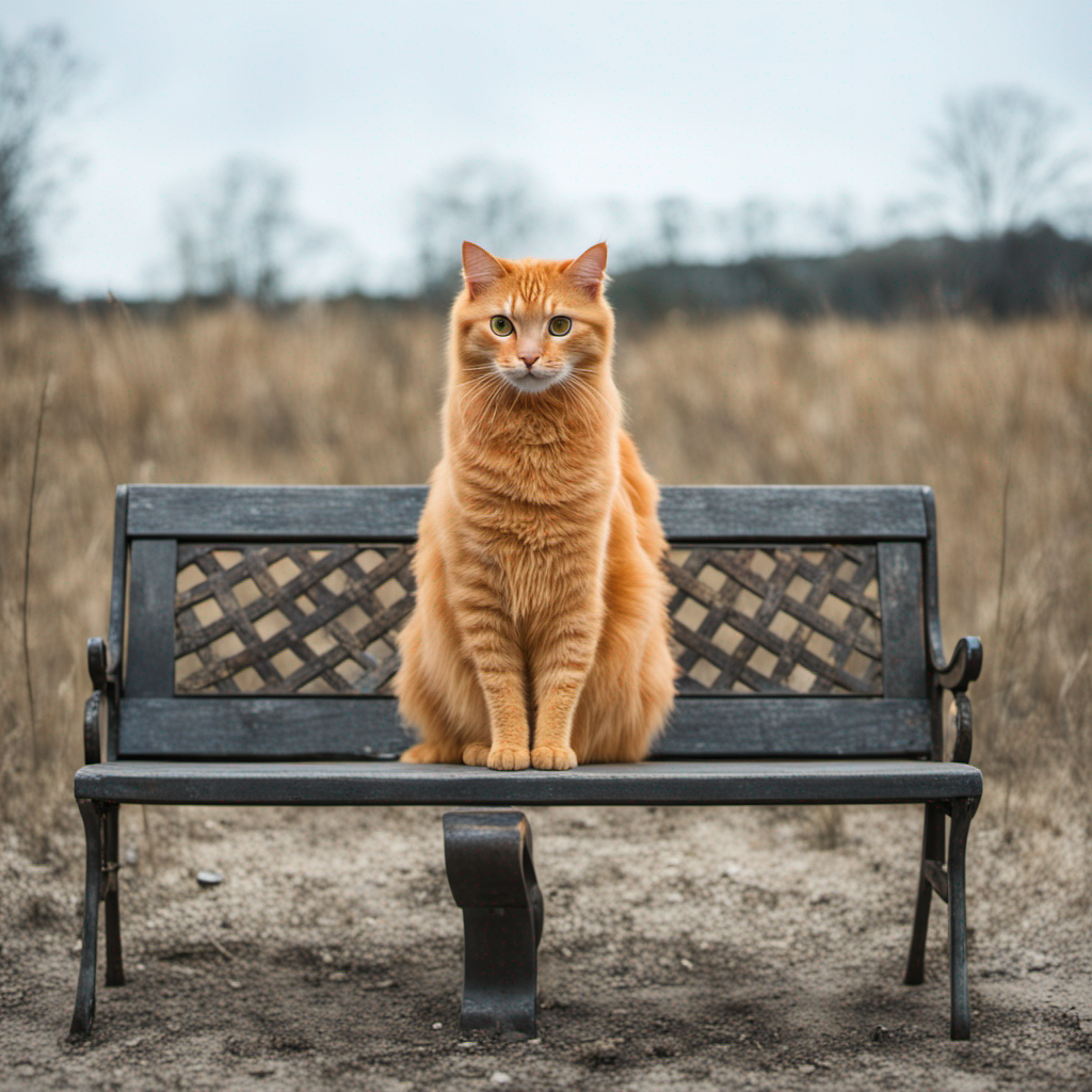
In the example below, you can see the difference – the cat is no longer dependent on the white-ish color of the dog – it is now much more orange as specified in the prompt.
In this guide, we’ve covered how to use inpainting to remove unwanted objects from an image, replace or change existing objects in an image, and fix ugly or broken parts of a previously generated image. But you can also use it to expand the canvas of an image. Check out the outpainting guide to learn more about that process.
Inpainting vs outpainting
Outpainting expands the canvas of an image. Consider a portrait photo where the top of the head is cropped out. Outpainting can be used to generate the missing part of the head.
It’s very similar to inpainting. But instead of generating a region within an existing image, the model generates a region outside of it. Learn more about outpainting.
Outpainting with Stable Diffusion
Outpainting is the process of using an image generation model like Stable Diffusion to extend beyond the canvas of an existing image. Outpainting is very similar to inpainting, but instead of generating a region within an existing image, the model generates a region outside of it.
Here’s an example of an outpainted image:
| Input | Output |
|---|---|
 |  |
In this guide, we’ll walk you through the process of creating your own outpainted images from scratch using Stable Diffusion SDXL.
Check out outpainter.app to easily generate your own outpainted images.
The outpainting process
At a high level, outpainting works like this:
- Choose an existing image you’d like to outpaint.
- Create a source image that places your original image within a larger canvas.
- Create a black and white mask image.
- Use your source image, your mask image, and a text prompt as inputs to Stable Diffusion to generate a new image.
🍿 Watch our inpainting and outpainting guide on YouTube
Step 1: Find an existing image
The first step is to find an image you’d like to outpaint. This can be any image you want, like a photograph, a painting, or an image generated by an AI model like Stable Diffusion.
Here’s an example of an image to outpaint, an AI-generated armchair in the shape of an avocado:
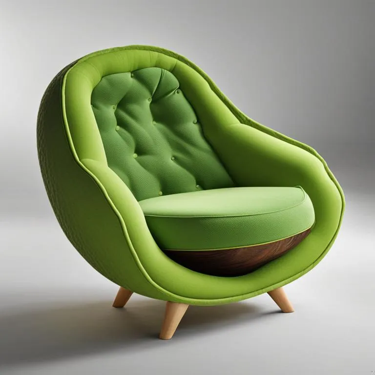
The image here has square dimensions, but your image can have any aspect ratio.
Step 2: Create a source image
Once you’ve found an image you want to outpaint, you need to place it within a larger canvas so the image model will have space to paint around it. You can do this with traditional raster image editing software like Photoshop or GIMP, but since you won’t actually be doing any manual bitmap-based editing of the image, you can also use web-based vector drawing tools like Figma or Canva to achieve the same result.
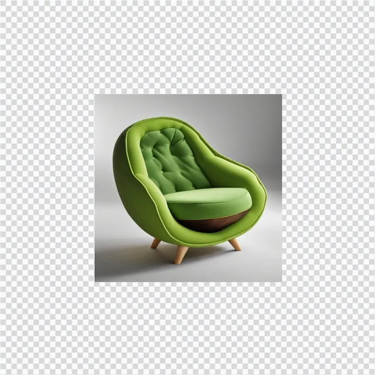
Create a new square image, and place your original image within it. 1024x1024 is ideal if you’re using the SDXL version of Stable Diffusion, as you will in this guide. For more info about image sizing and dimensions, see the docs on width and height.
In the example image below, there’s a checkboard pattern to indicate the “transparent” parts of the canvas that will be outpainted, but the checkboard is not actually necessary. You can choose any color you like for the surrounding canvas, but it’s a good idea to choose a color that’s similar to the color of the image you’re outpainting. This will help the model generate a more seamless transition between the original image and the outpainted region.
It should look something like this:
☝️ Here the original image is centered in the middle of the canvas, but you can place it anywhere you like depending on which part of the canvas you’d like to outpaint. These are also perfectly valid arrangements:
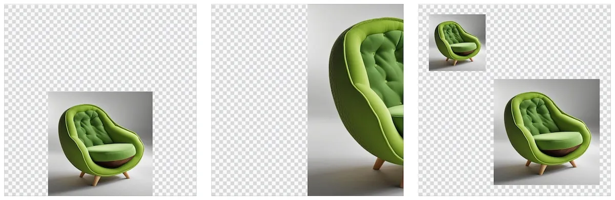
Save this image as a JPG or PNG file. Give it a name like outpainting-source.jpg or outpainting-source.png so you can easily identify it later.
Step 3: Create a mask image
Next, you’ll generate a mask image. This is a black and white image that tells the model which parts of the image to preserve, and which parts to generate new content for. Again you can use any image editing tool you like do to do this, as long as it can save JPG or PNG files.
Use the same dimensions for your mask image as you did for your source image: 1024x1024 square. The mask image should be black and white, with the black areas representing the parts of the image you want preserve, and the white areas representing the parts of the image you want to generate new content for.
If you can’t easily remember which parts should be black and which should be white, try asking ChatGPT to create a mnemonic for you. Here’s one:
Keep the Night, Replace the Light
For our centered avocado armchair, the mask image should look something like this:
☝️ Important! Be sure to draw your mask slightly smaller than the source image. This will help the model generate a more seamless visual transition between the original image and the outpainted region. It will also prevent an unwanted visible line from being drawn between the original image and the outpainted region.
Save this image as a JPG or PNG file. Give it a name like outpainting-mask.jpg or outpainting-mask.png so you can easily identify it later.
Step 4: Generate the outpainted image
Now that you’ve generated your source image and mask image, you’re ready to generate the outpainted image. There are many models that support outpainting, but in this guide you’ll use the SDXL version of Stable Diffusion to generate your outpainted image.
The inputs you’ll provide to stable diffusion are:
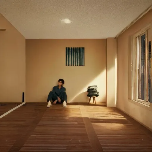
prompt: A short string of text describing the image you’d like to generate. To see what your avocado armchair would look like if it were in a larger room, use a prompt like “an armchair in a room full of plants”.image: The source image you created in step 2.mask: The mask image you created in step 3.
Use Replicate’s web interface
To generate your outpainted image using Replicate’s web interface, follow this link, replacing the image, mask, and prompt inputs with your own values. The web UI makes it easy to drag and drop your image and mask files right into the browser window.
Use Replicate’s API
To generate your outpainted image using Replicate’s API, you can use whatever programming language you prefer, but in this guide we’ll use Python.
Start by setting up the Python client, then run this code:
import replicate
output = replicate.run(
  "stability-ai/sdxl:39ed52f2a78e934b3ba6e2a89f5b1c712de7dfea535525255b1aa35c5565e08b",
  input={
    "prompt": "an armchair in a room full of plants",
    "image": open("path/to/outpainting-source.jpg", "rb"),
    "mask": open("path/to/outpainting-mask.jpg", "rb")
  }
)

# Save the outpainted image
with open('outpainted.png', 'wb') as f:
    f.write(output[0].read())
The resulting image should look something like this:
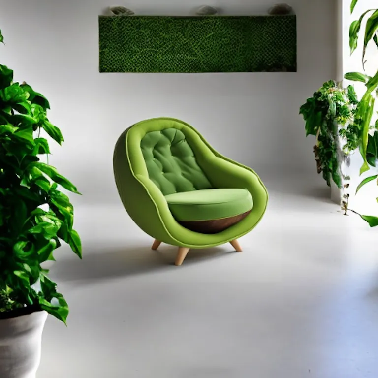
Now that you’ve generated your first outpainted image, it’s time to iterate. Refine the prompt, adjust the mask, and try again. This is where the API really shines, because you can easily write code to run the model multiple times with different inputs to see what works best.
Happy outpainting! 🥑
Fine-tuning Stable Diffusion
You can fine-tune Stable Diffusion on your own images to create a new version of the model that is better at generating images of a person, object, or style.
For example, we’ve fine-tuned SDXL on:
Types of fine-tune
There are multiple ways to fine-tune Stable Diffusion, such as:
- Dreambooth
- LoRAs (Low-Rank Adaptation)
- Textual inversion
Each of these techniques need just a few images of the subject or style you are training. You can use the same images for all of these techniques. 5 to 10 images is usually enough.
Dreambooth
Dreambooth is a full model fine-tune that produces checkpoints that can be used as independent models. These checkpoints are typically 2GB or larger.
Read our blog post for a guide on using Replicate for training Stable Diffusion with Dreambooth.
Google Research announced Dreambooth in August 2022 (read the paper).
LoRAs (Low-Rank Adaptation)
LoRAs are faster to tune and more lightweight than Dreambooth. As small as 1-6MB, they are easy to share and download.
LoRAs are a general technique that accelerate the fine-tuning of models by training smaller matrices. These then get loaded into an unchanged base model to apply their affect. In February 2023 Simo Ryu published a way to fine-tune diffusion models like Stable Diffusion using LoRAs.
You can also use a lora_scale to change the strength of a LoRA.
Textual inversion
Textual inversion does not modify any model weights. Instead it focuses on the text embedding space. It trains a new token concept (using a given word) that can be used with existing Stable Diffusion weights (read the paper).
Fine-tuning SDXL using Replicate
You can fine-tune SDXL using Replicate – these fine-tunes combine LoRAs and textual inversion to create high quality results.
There are two ways to fine-tune SDXL on Replicate:
- Use the Replicate website to start a training, you can change the most important training parameters
- Use the Replicate API to train with the full range of training parameters
Whichever approach you choose, you’ll need to prepare your training data.
Prepare your training images
When running a training you need to provide a zip file containing your training images. Keep the following guidelines in mind when preparing your training images.
Images should contain only the subject itself, without background noise or other objects. They need to be in JPEG or PNG format. Dimensions, file size and filenames don’t matter.
You can use as few as 5 images, but 10-20 images is better. The more images you use, the better the fine-tune will be. Small images will be automatically upscaled. All images will be cropped to square during the training process.
Put your images in a folder and zip it up. The directory structure of the zip file doesn’t matter:
zip -r data.zip dataWatch the API fine-tuning guide on YouTube
Use the Replicate CLI to start a training
This guide uses the Replicate CLI to start the training, but if you want to use something else you can use a client library or call the HTTP API directly.
Let’s start by installing the Replicate CLI:
brew tap replicate/tap
brew install replicate
Grab your API token from replicate.com/account and set the REPLICATE_API_TOKEN environment variable.
export REPLICATE_API_TOKEN=...You need to create a model on Replicate – it will be the destination for your trained SDXL version:
# You can also go to https://replicate.com/create
replicate model create yourname/model --hardware gpu-a40-small
Now you can start your training:
replicate train stability-ai/sdxl \
 --destination yourname/model \
 --web \
 input_images=@data.zip
The input_images parameter is required. You can pass in a URL to your uploaded zip file, or use the @ prefix to upload one from your local filesystem.
See the training inputs on the SDXL model for a full list of training options.
Visit replicate.com/trainings to follow the progress of your training job.
Run the model
When the model has finished training you can run it using replicate.com/my-name/my-model, or via the API:
output = replicate.run(
    "my-name/my-model:abcde1234...",
    input={"prompt": "a photo of TOK riding a rainbow unicorn"},
)

# Save the generated image
with open('output.png', 'wb') as f:
    f.write(output[0].read())
The trained concept is named TOK by default, but you can change that by setting token_string and caption_prefix inputs during the training process.
How we prepare data for training
Before fine-tuning starts, the input images are preprocessed using multiple models:
- SwinIR upscales the input images to a higher resolution.
- BLIP generates text captions for each input image.
- CLIPSeg removes regions of the images that are not interesting or helpful for training.
For most users, the captions that BLIP generates for training work well. However, you can provide your own captions by adding a caption.csv file to your zip file of input images. Each image needs a caption. Here’s an example csv.
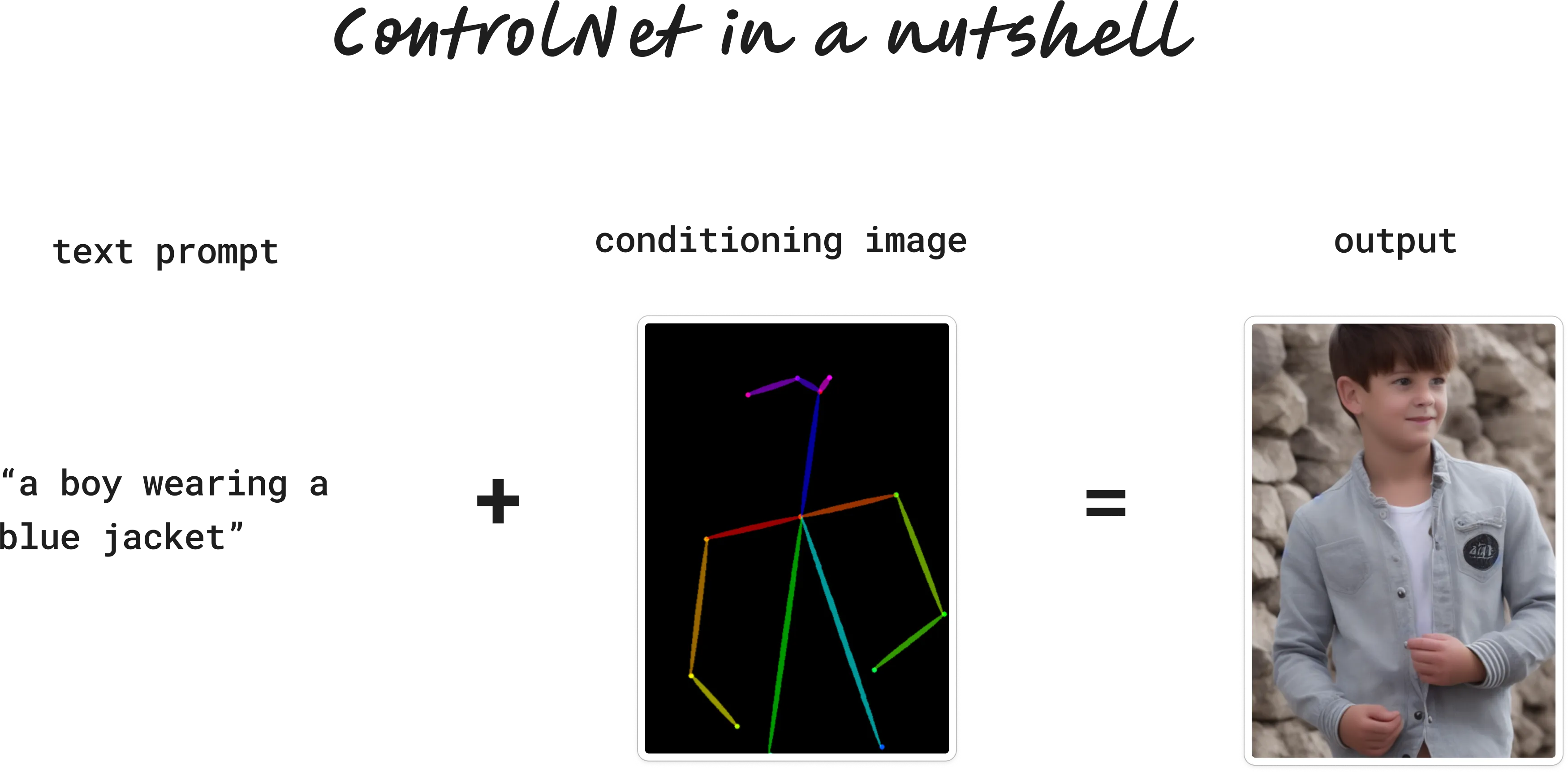
Using ControlNet with Stable Diffusion
ControlNet is a method for conforming your image generations to a particular structure. It’s easiest explained by an example.
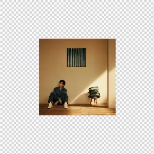
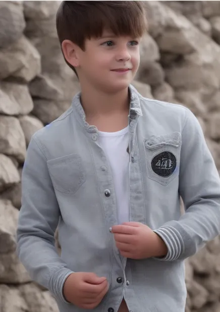
Let’s say you wanted to create an image of a particular pose—a photo like the man below, but we want a boy doing it.
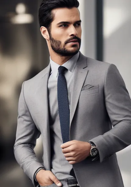
This is a really hard problem with default stable diffusion. We could try a prompt that describes our desired pose in detail, like this:
a photo of a boy wearing a blue jacket looking to his right with his left arm slightly above his right
But this probably isn’t going to work. Our outputs aren’t going to conform to all these instructions, and even if we got lucky and they did, we won’t be able to consistently generate this pose. (why? — my guess is because the decoder can only conform to so much? or maybe this is possible, it’s just a pain?)
Enter ControlNet. ControlNet models accept two inputs:
A text prompt: a boy wearing a blue jacket
And a conditioning image. There are lots of types, but for now let’s use a stick figure (often called human pose):
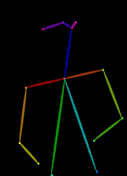
The model then uses our pose to conform/shape/control our image into our desired structure:
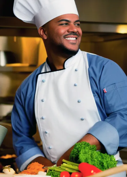
Let’s try changing our prompt, but keep the pose input the same:
“chef in kitchen”
“Lincoln statue”
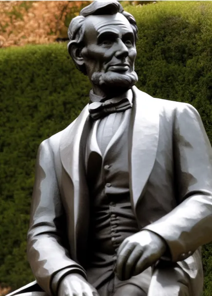
Source: ControlNet paper
And voila! We can create all kinds of images that are guided by the stick figure pose.
That’s the essence of ControlNet. We always provide two inputs: a text prompt (just like normal Stable Diffusion) and a conditioning image. The output is guided by our conditioning image.
Importantly, the conditioning image isn’t restricted to stick figure poses. We can provide all kinds of custom compositions for the ControlNet model to follow, like edges, depths, scribbles, segmentation and many other structures. More on that later.
How does ControlNet work?
ControlNet was created by Stanford researchers and announced in the paper Adding Conditional Control to Text-to-Image Diffusion Models.
It’s trained on top of stable diffusion, so the flexibility and aesthetic of stable diffusion is still there.
I don’t want to go too in depth, but training ControlNet involves using conditioning images to teach the model how to generate images according to specific conditions. These conditioning images act like guidelines or templates. For example, if the model is to learn how to generate images of cats, it might be trained with a variety of images showing cats in different poses or environments. Alongside these images, text prompts are used to describe the scene or the object. This combination of visual and textual input helps the model understand not just what to draw (from the text) but also how to draw it (from the conditioning images).
To learn more, check out the paper. Or do what I did, and upload the paper to ChatGPT and ask it a bunch of questions.
Types of conditioning images
Watch this section on YouTube
There are many types of conditioning_image’s we can use in ControlNet. We’re not restricted to our human pose. We can guide our images using edge detectors, depth maps, segmentation, sketchs, and more.
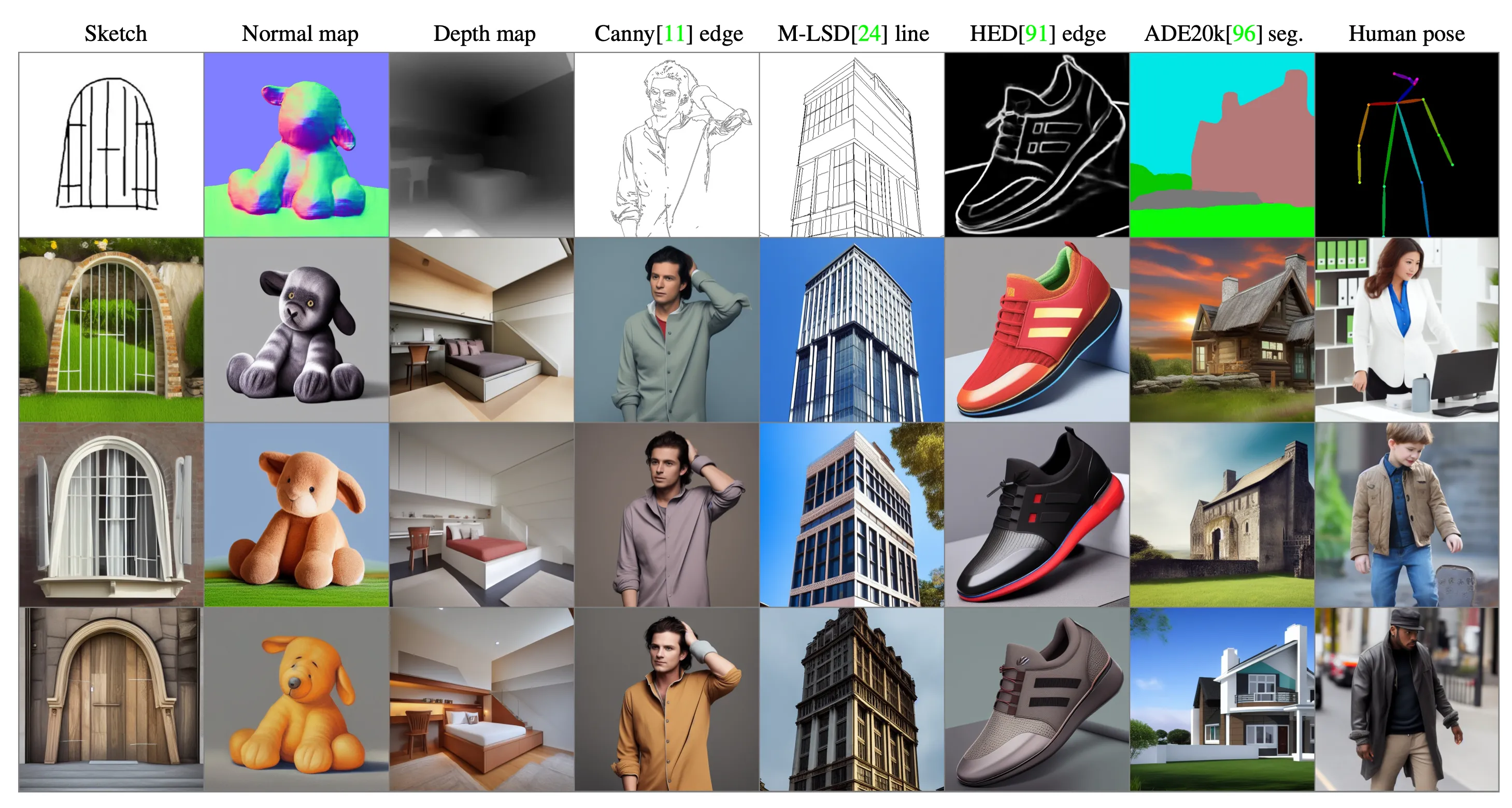
The best way to see how each of these work is by example.
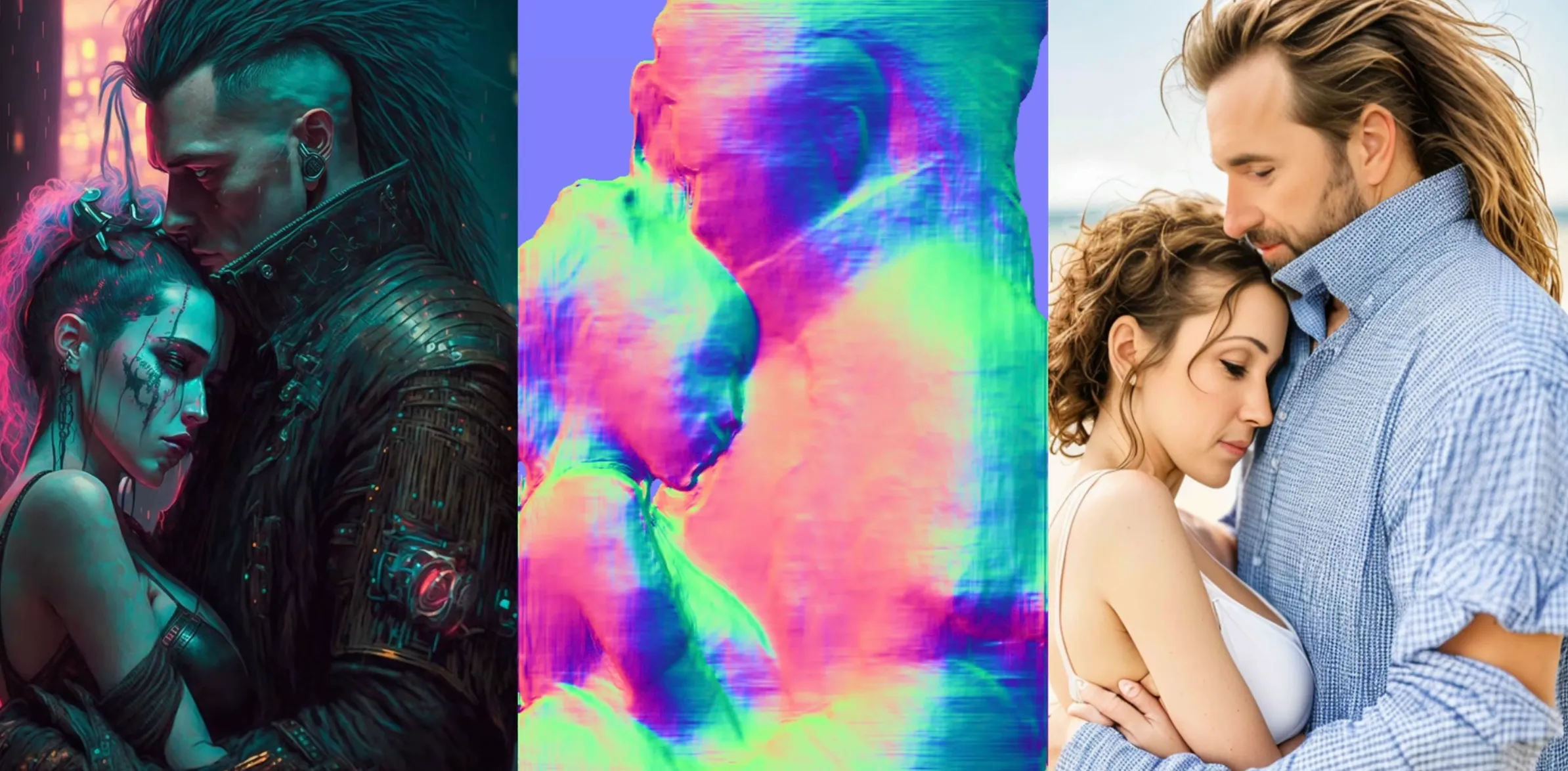
Let’s run a selection of conditioners on the following two images with completely new prompts.
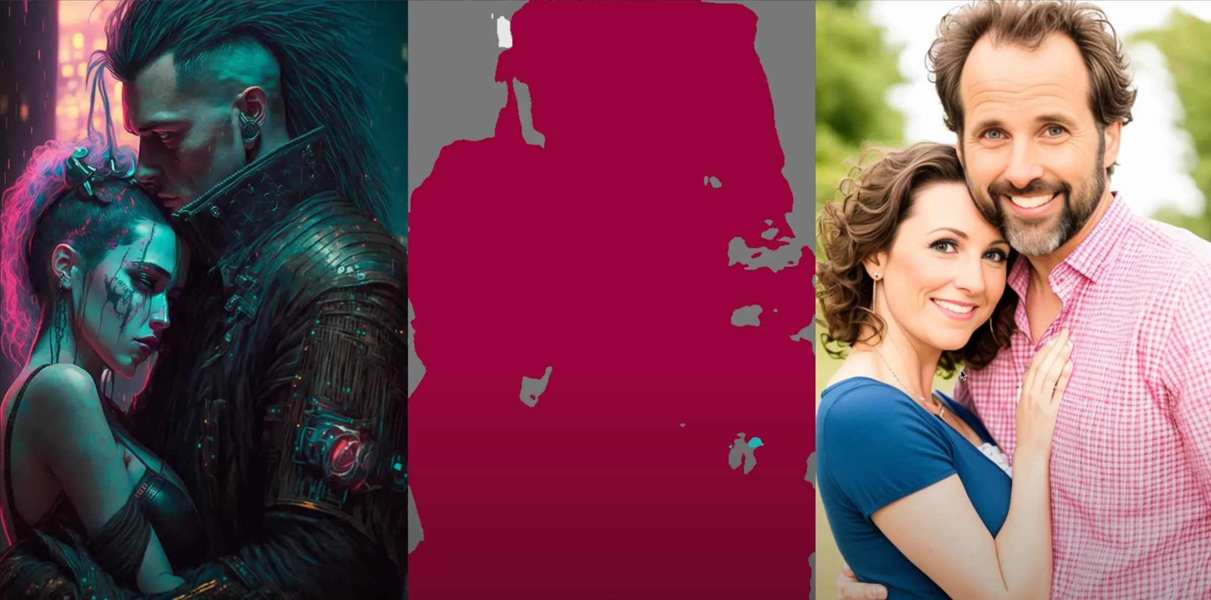
Cyberpunk Couple New prompt:
a portrait photo of a thirtysomething
couple embracing, summer clothes,
color photo, 50mm prime, canon, studio
portrait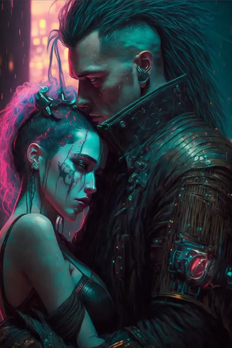
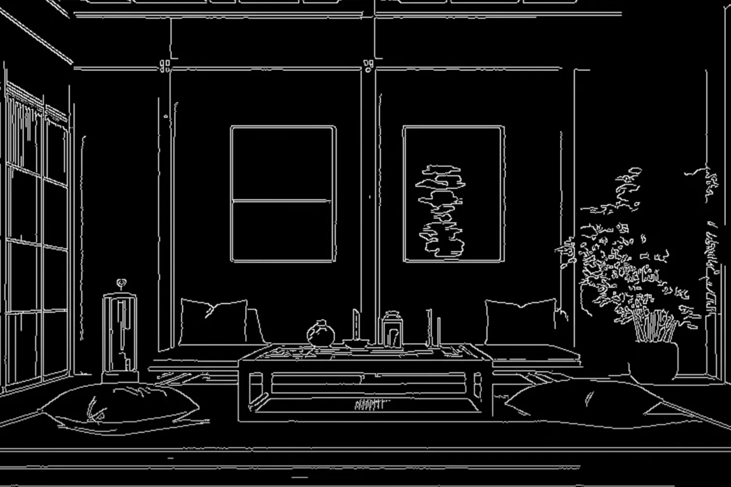
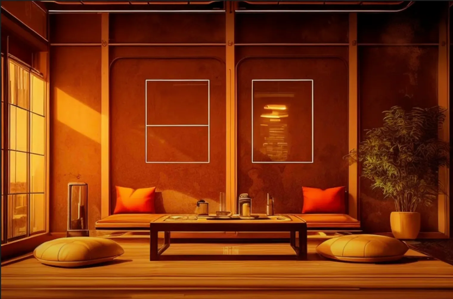
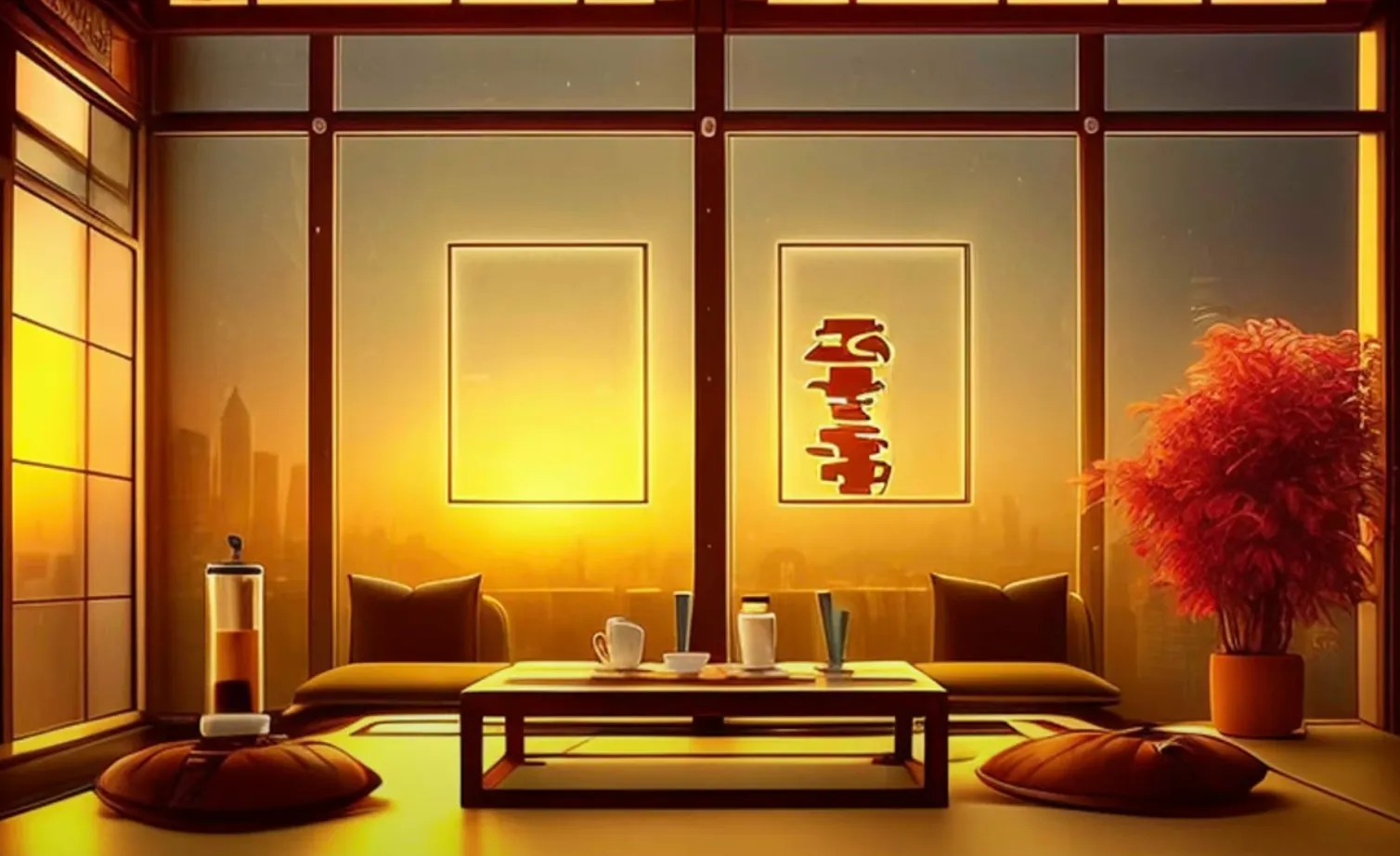
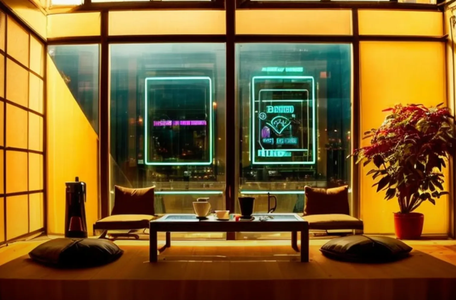
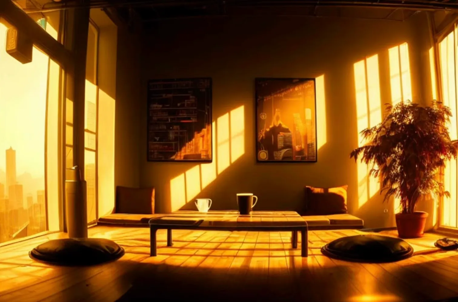
Tea Room New prompt:
a photo of a beautiful cyberpunk
cafe, dawn light, warm tones,
morning scene, windows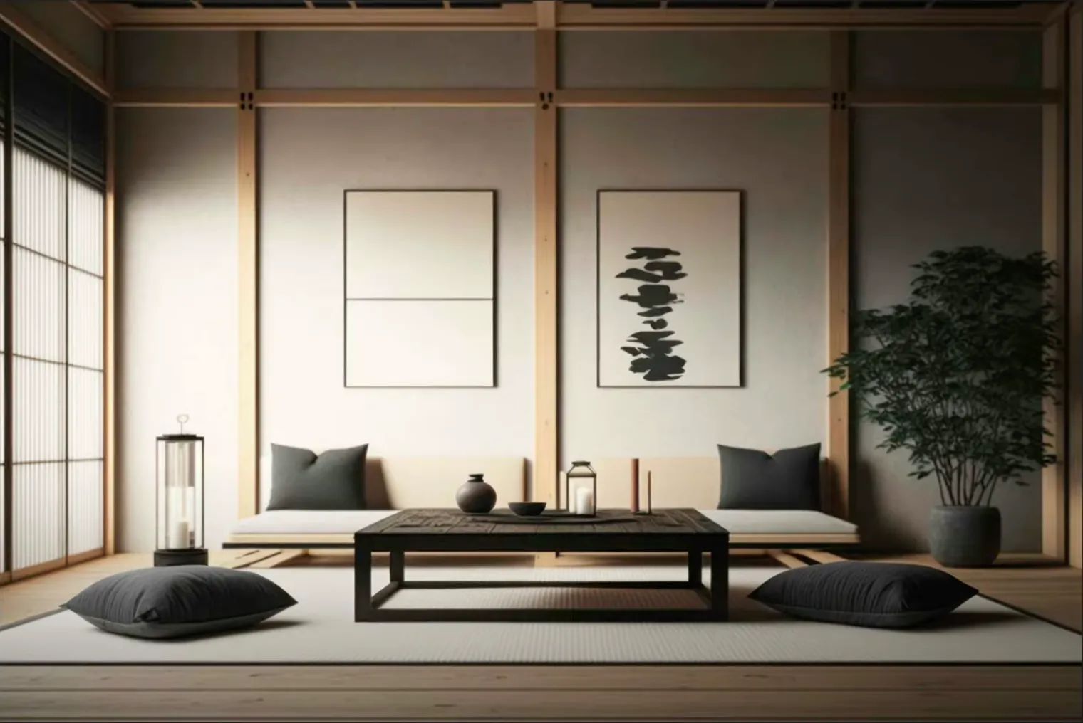
Let’s see what happens when we apply different ControlNets on these two images. In other words, let’s go through this process for each type of conditioner:
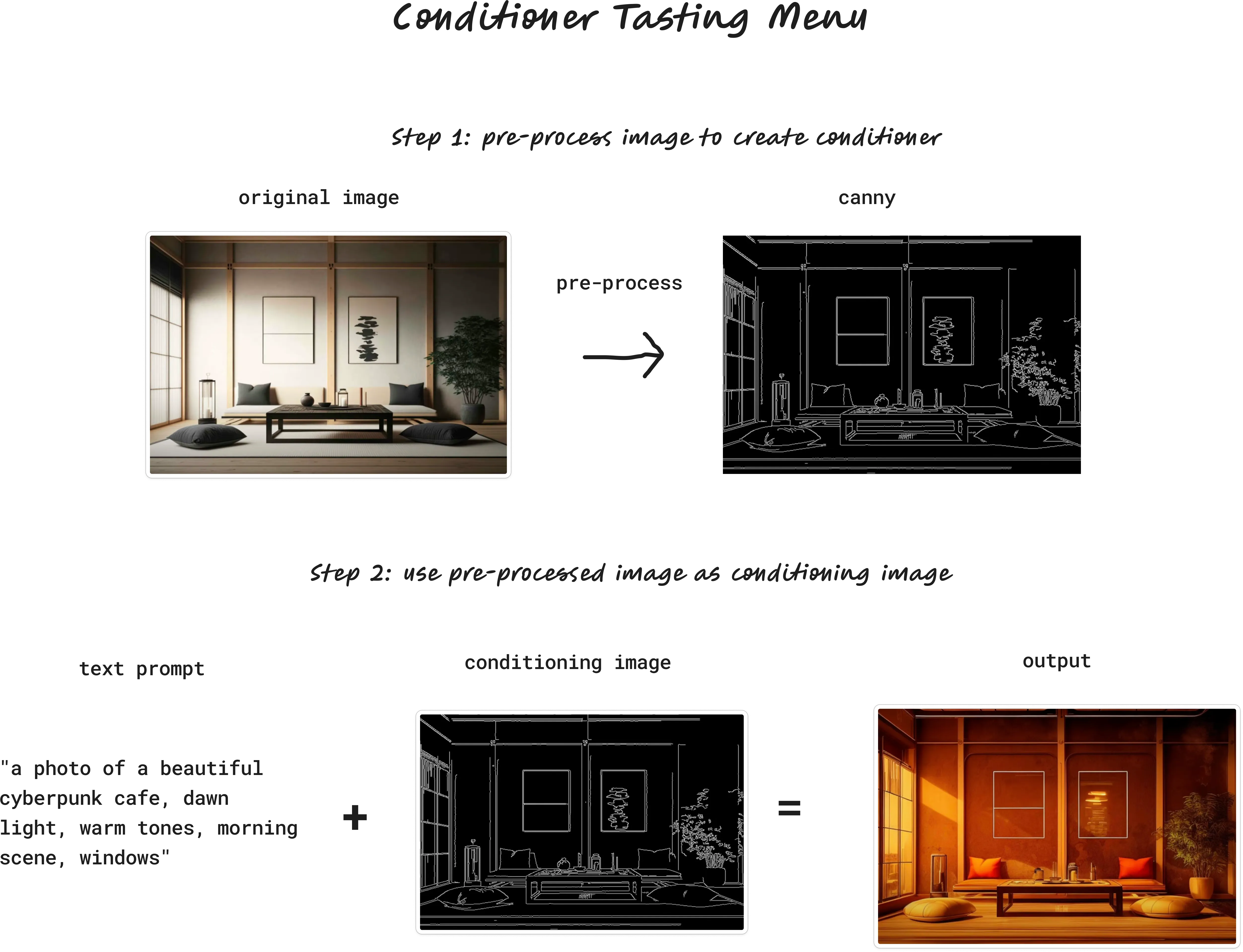
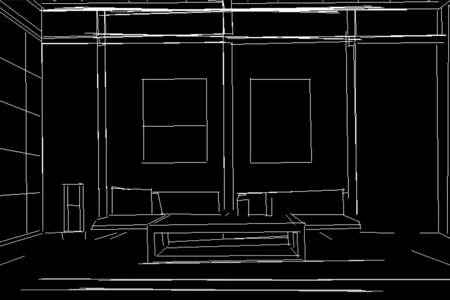
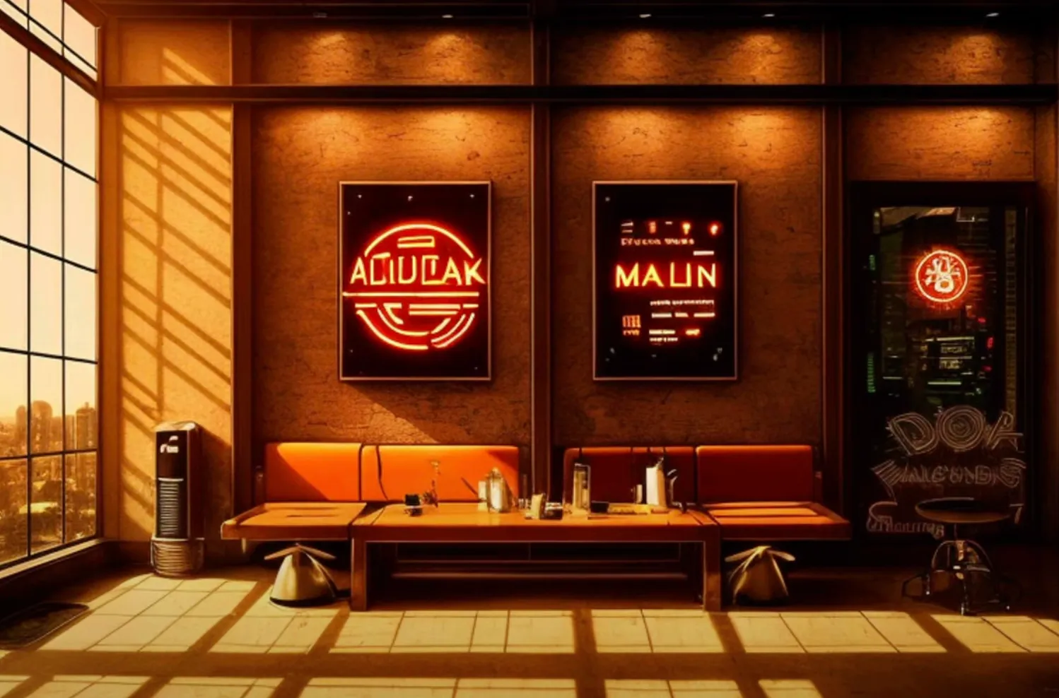
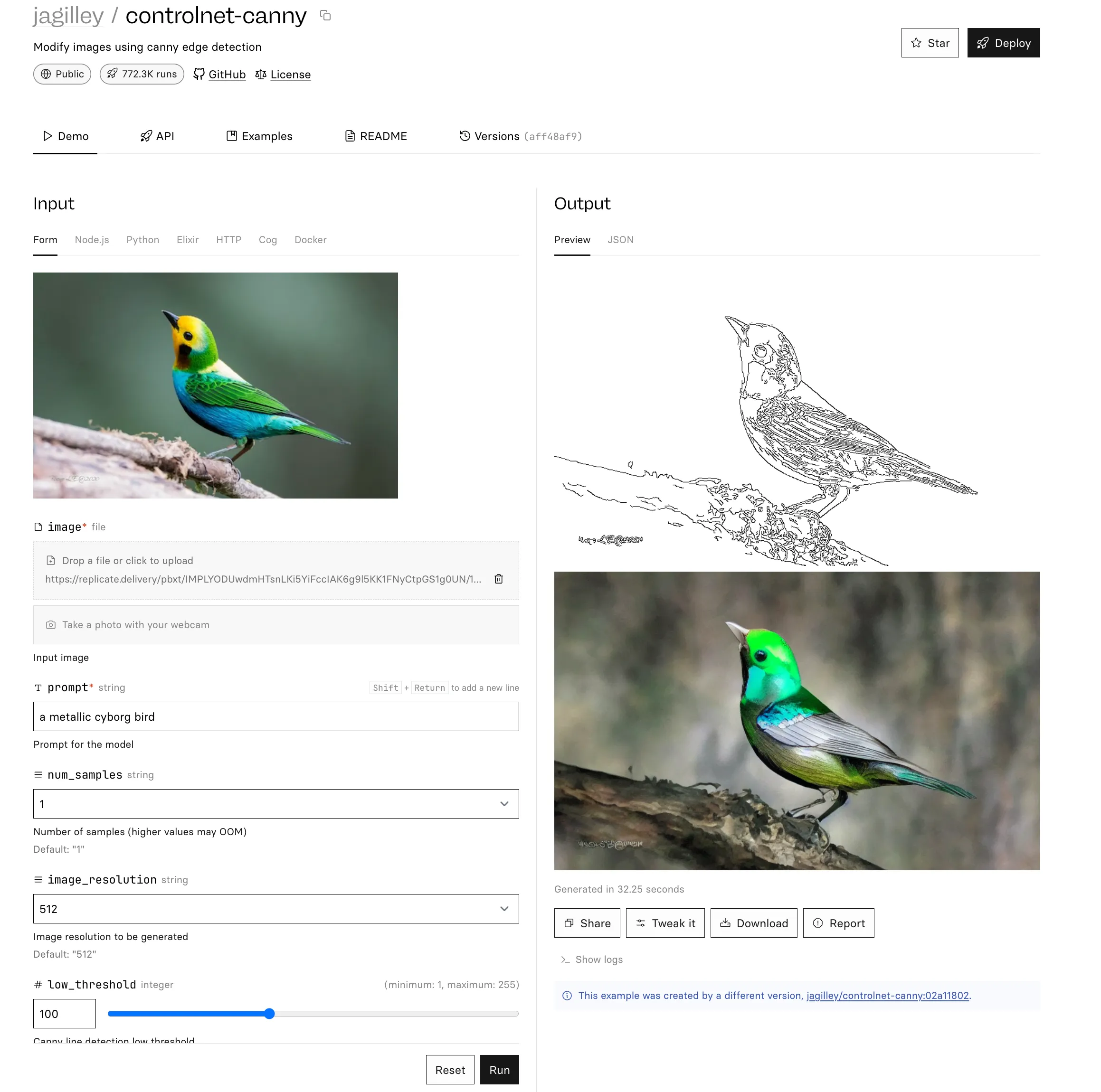
Canny — Edge detection
Canny is a widely used edge detector.
Here’s our tea room after going through the Canny pre-processor:
Remember our prompt from earlier?
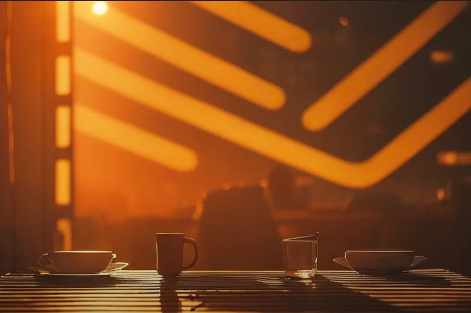
"a photo of a beautiful cyberpunk
cafe, dawn light, warm tones,
morning scene, windows"
Now, when we generate an image with our new prompt, ControlNet will generate an image based on this prompt, but guided by the Canny edge detection: Result
Here’s that same process applied to our image of the couple, with our new prompt:
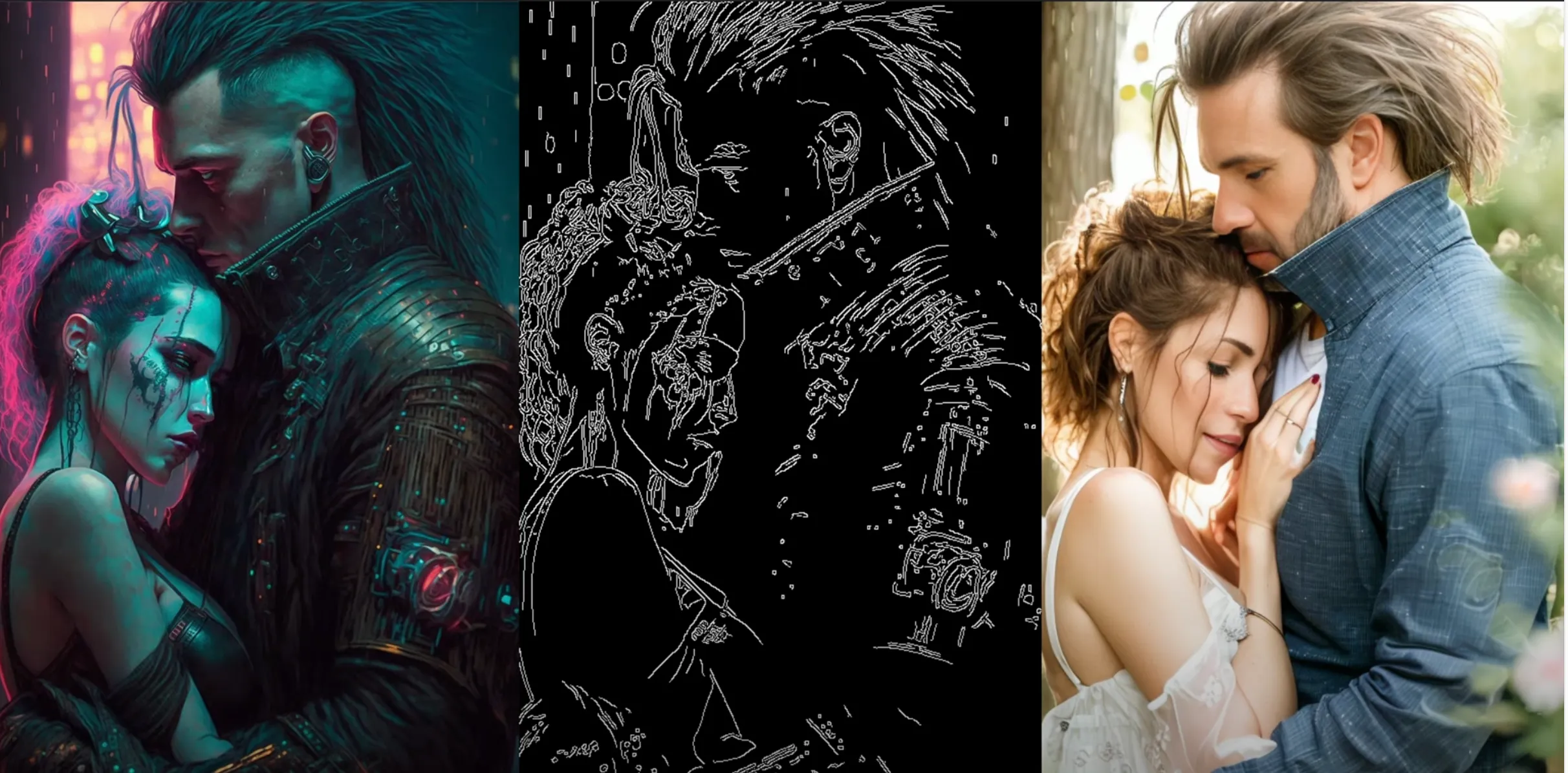
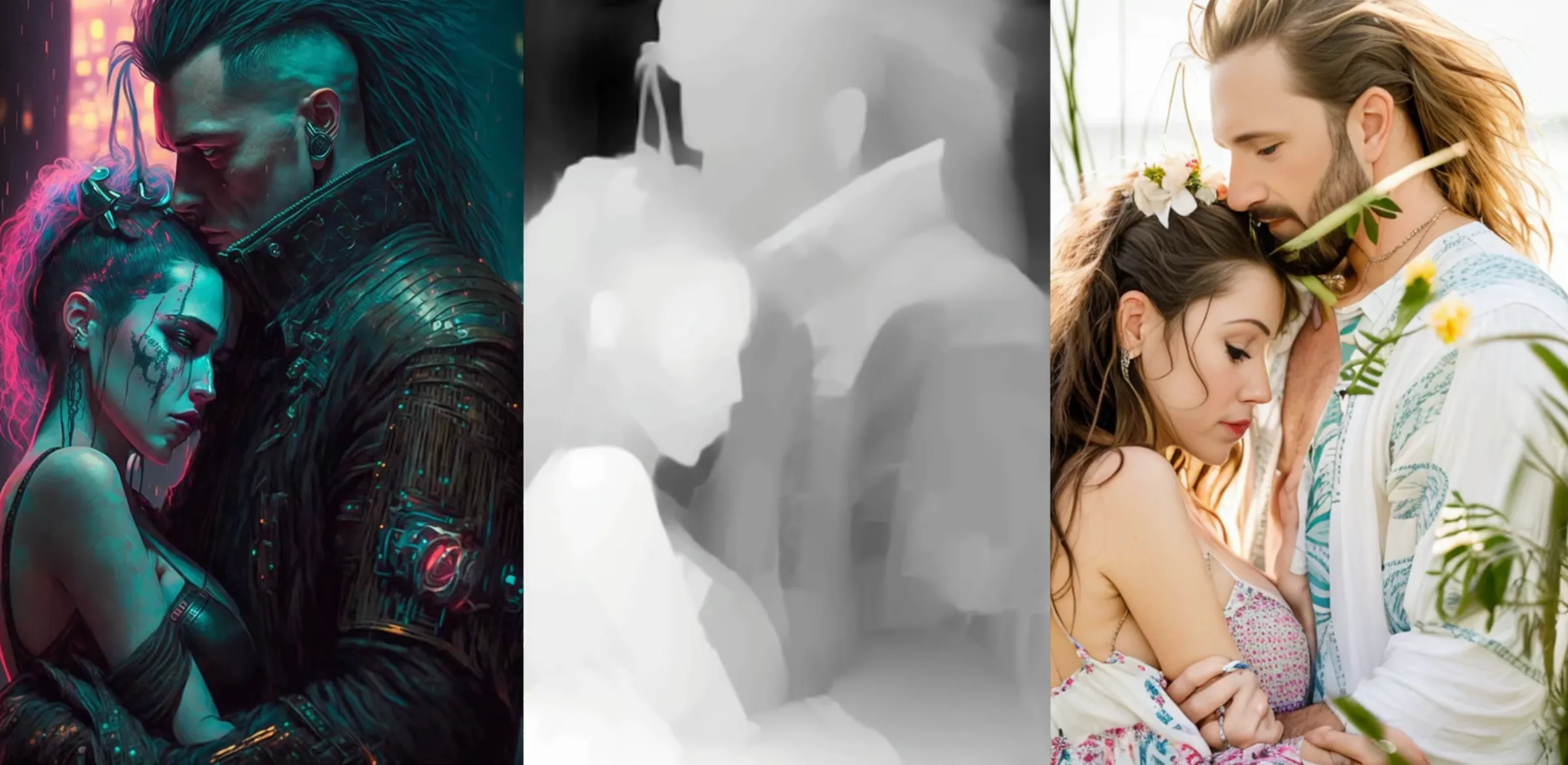
HED — Fuzzy edge detection
HED is another kind of edge detector. Here’s our pre-processed output:
And here’s our output:
The effect of HED is a bit more clear on our cyberpunk couple:
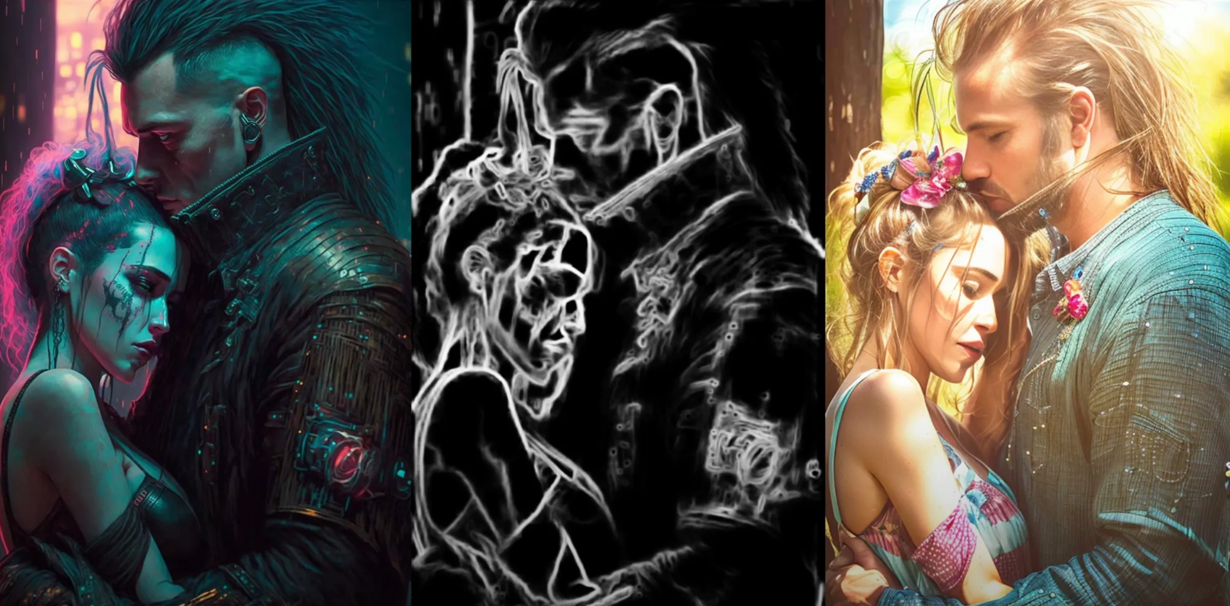
Note that many details that were lost in the Canny version are present in HED detection, like her hand placement, the angle of the overhead light, and her headpiece. Note also where HED struggles—his collar becomes a streak of hair, and her makeup becomes a shadow. HED works really well for painting and art.
M-LSD — Straight line detection
M-LSD is another kind of edge detection that only works on straight lines. Here’s M-LSD on our tea room:
And on our cyberpunk couple:
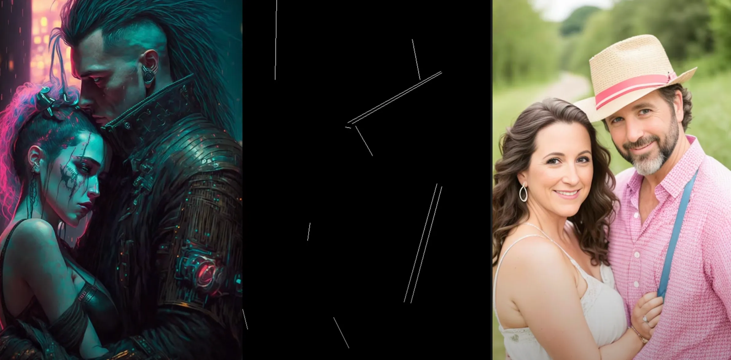
As you can tell, M-LSD doesn’t work well here—there aren’t many straight lines in the original.
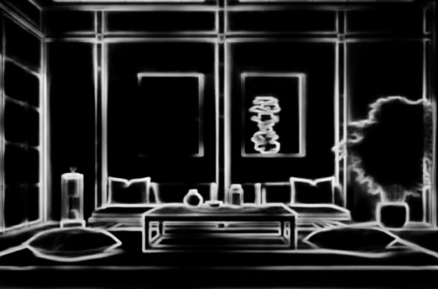
Depth Map
A depth map works by simulating the distance of parts of the image from the camera. Here’s what it looks like:
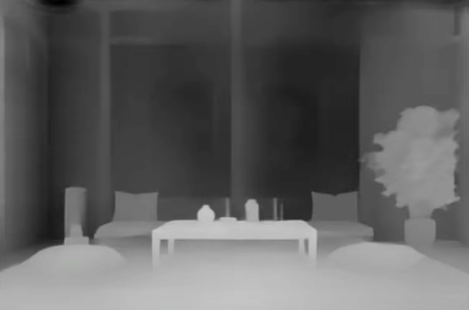
This works really well on our tea room. The frames, plants, tables and pillows are all preserved. Let’s try it on our couple:
Again, the composition is preserved, but it struggles with the collar and hands.
Open pose (aka Human pose)
This one should be familiar to you! Open pose/human pose turns images of people into stick figures. Let’s try it on our couple:
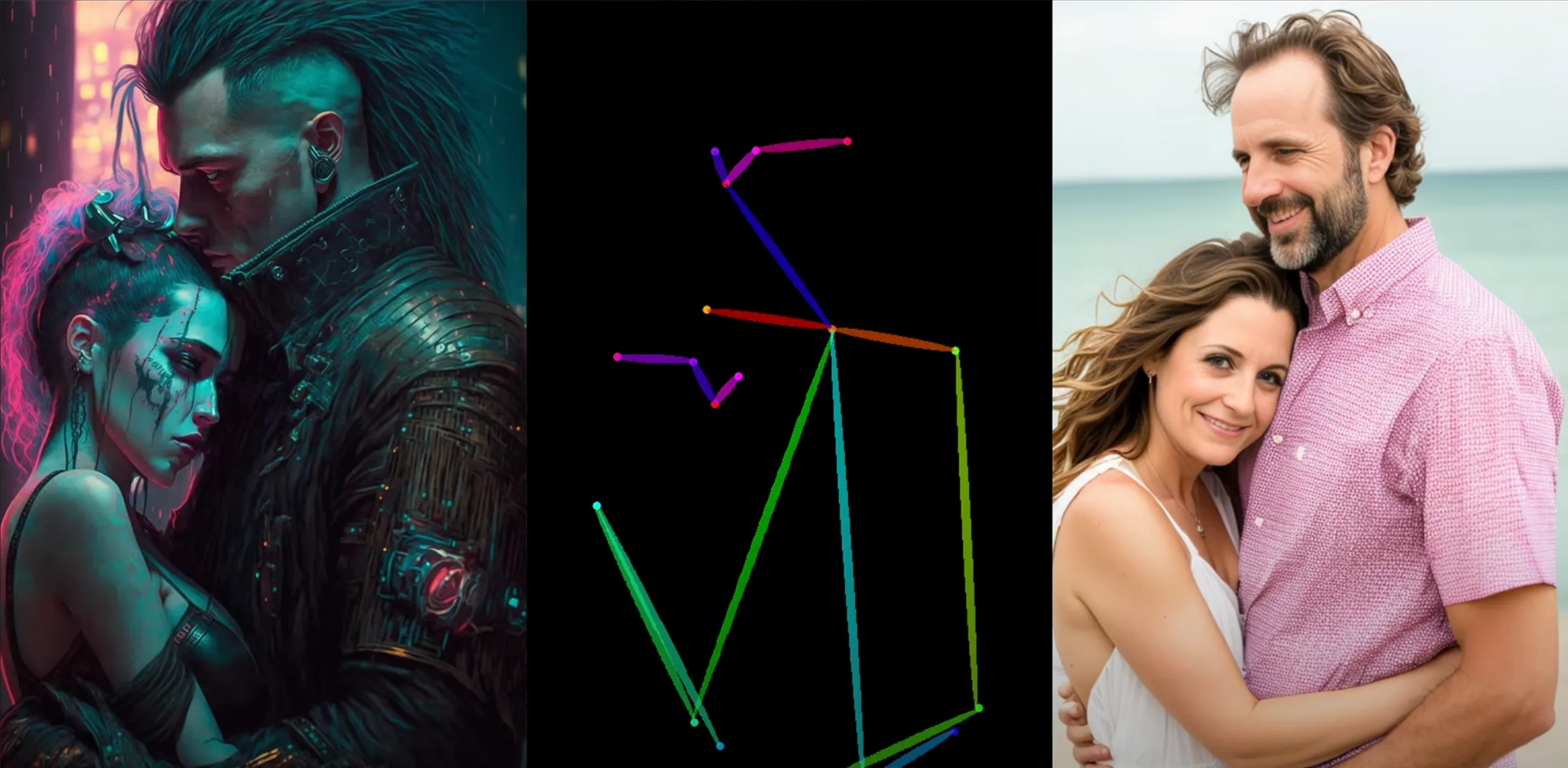
The colored bars are representations of the body parts of our characters. You can see that the poses are preserved, but the detail and style is lost.
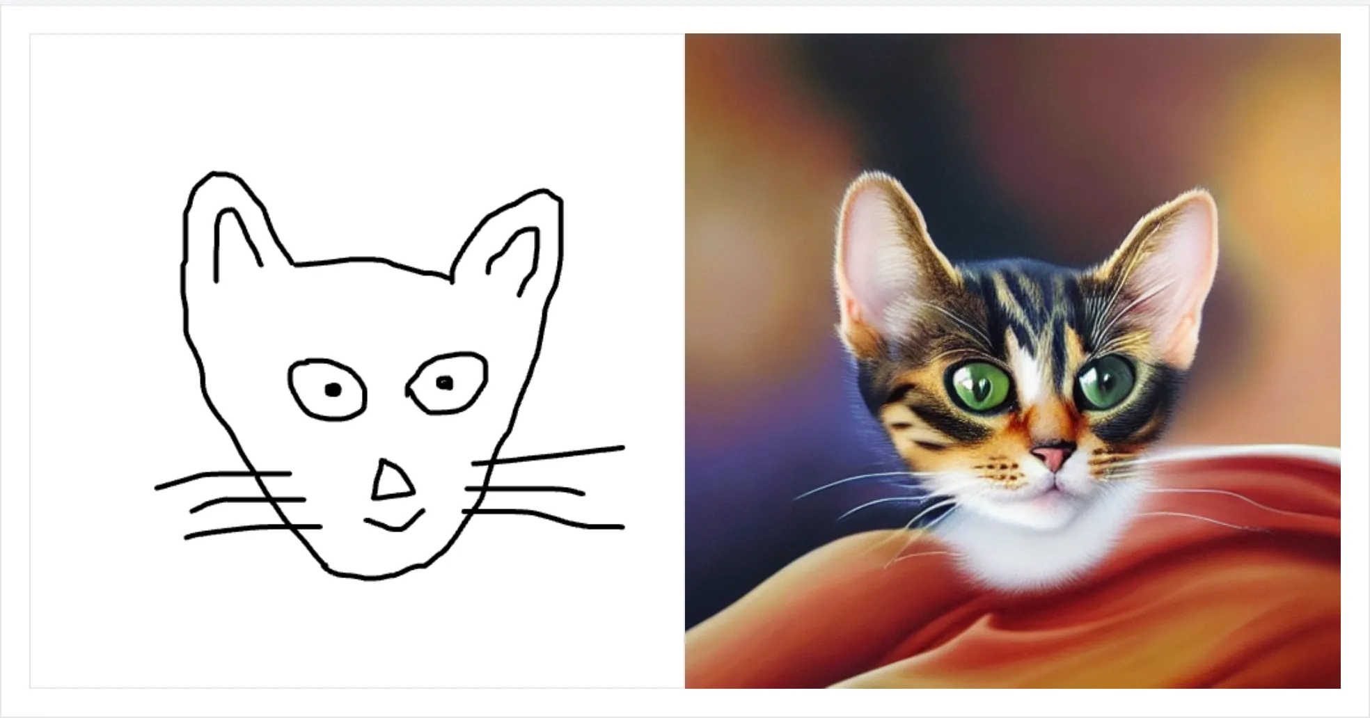
Scribble
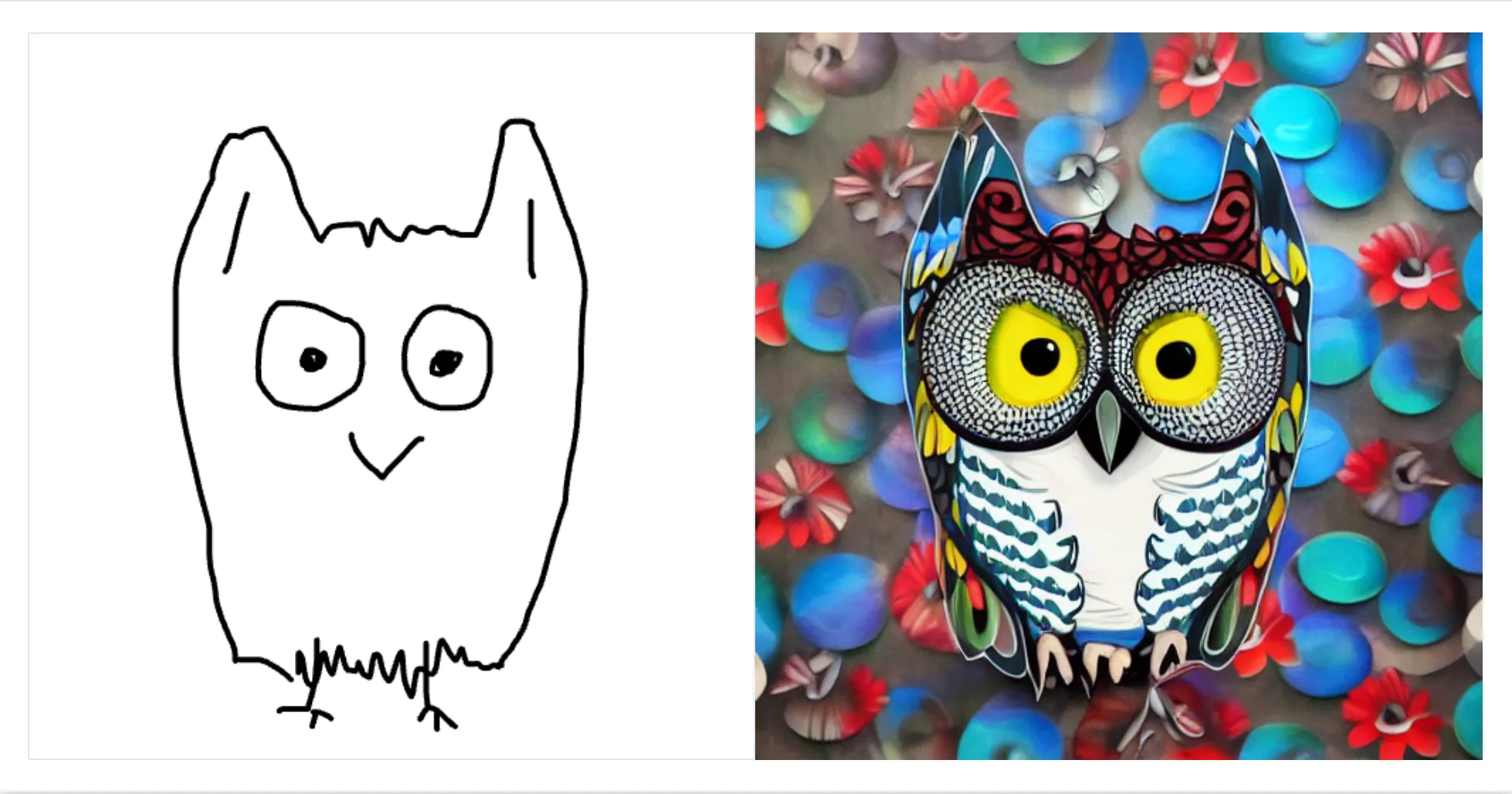
Scribble is behind the very popular “turn a sketch into a drawing” apps. I’m going to use a different example for scribble, because it works best with a doodle input conditioner. For example, here’s a doodle of a cat alongside my text prompt, “an oil painting of a cat”:
Here’s the same with an owl:
Segmentation
Segmentation breaks our image down into different segments.
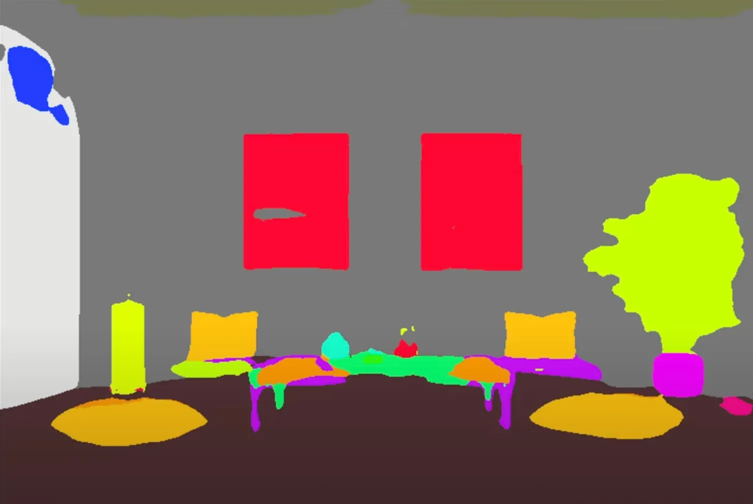
We’ve maintained the plants, the frames, and the table, but the output is quite different. There’s a bit of a fish eye effect, and we’ve lost the pillars in the cafe. Here’s segmentation on our couple.
Normal map
A normal map detects the texture of an image.
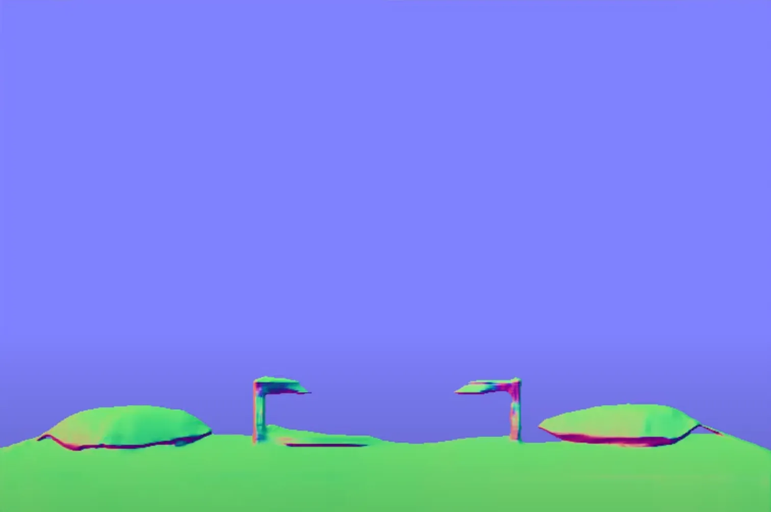
This is a nice output, but it doesn’t preserve our original input at all. A normal map works much better on our couple:
How to use ControlNet
Using ControlNet is easy with Replicate 😎. We have a collection of ControlNet models here.
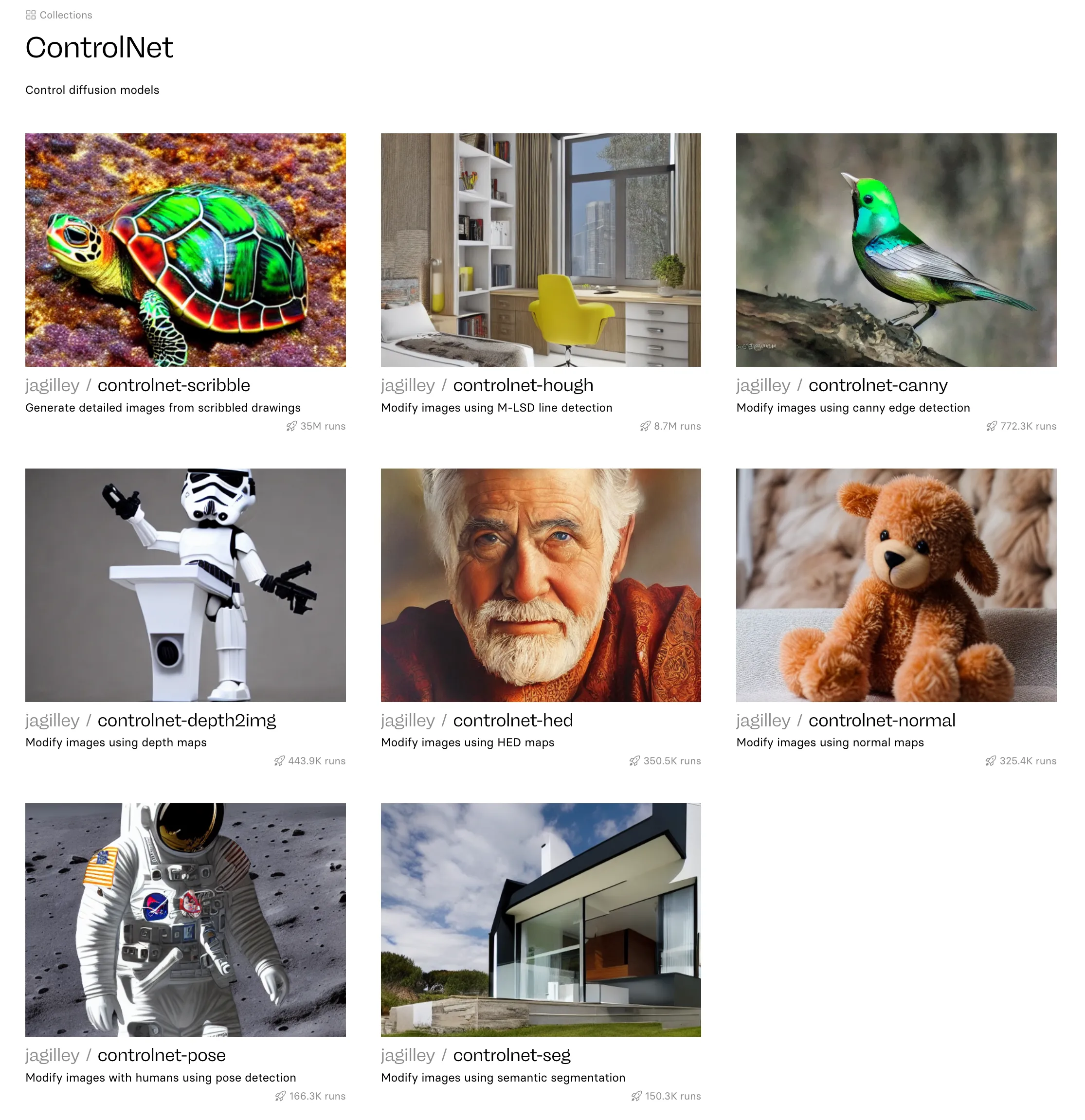
You can get started by choosing a ControlNet model and playing around with it in our GUI. If you’re a developer and want to integrate ControlNet into your app, click the API tab and you’ll be able to copy and paste the API request into your codebase. Happy hacking!
Fast Stable Diffusion: Turbo and latent consistency models (LCMs)
You might have noticed that Stable Diffusion is now fast. Very fast. 8 frames per second, then 70fps, now reports of over 100fps, on consumer hardware.
Today you can do realtime image-to-image painting, and write prompts that return images before you’re done typing. There’s a whole new suite of applications for generative imagery. And other models, like text-to-video, will soon apply these techniques too.
In this guide we’ll aim to explain the different models, terms used and some of the techniques that are powering this speed-up.
Let’s start with latent consistency models, or LCMs. They started it all, and they brought about the first realtime painting apps, like Krea AI popularised.
Latent consistency models (LCM)
In October 2023, Simian Luo et al. released the first latent consistency model and we blogged about how to run it on a Mac and make 1 image per second. You can also run it on Replicate.
What made it so fast is that it needs only 4 to 8 steps to make a good image. This compares with 20 to 30 for regular Stable Diffusion. LCMs can do this because they are designed to directly predict the reverse diffusion outcome in latent space. Essentially, this means they get to the good pictures faster. Dig into their research paper if you want to learn more.
The latent consistency model that was released, the one based on a Stable Diffusion 1.5 finetune called Dreamshaper, is very fast. But what about other models? How can we speed them up?
One of the big drawbacks with LCMs is the way these models are made – in a process called distillation. The LCM must be distilled from a pre-trained text to image model. Distillation is a training process that needs ~650K text-image pairs and 32 hours of A100 compute. The authors distillation code also hasn’t been released.
LoRAs to the rescue.
LCM LoRAs
In November 2023, a new innovation followed – Huggingface blogged about a way to get all the benefits of LCM for any Stable Diffusion model or fine-tune, without needing to train a new distilled model. Full details are in their paper.
They did this by training an “LCM LoRA”. A much faster training process that can capture the speed-ups of LCM by training just a few LoRA layers.
You can experiment with these LoRAs using models on Replicate:
Suddenly we have very fast 4 step inference for SDXL, SD 1.5, and all the fine tunes that go with them. On a Mac, where a 1024x1024 image would take upwards of 1 minute, it’s now ready in just 6 seconds.
There is a downside though. The images these LCM LoRAs generate are lower quality, and need more specific prompting to get good results.
You also need to use a guidance scale of 0 (ie turning it off) or between 1 and 2. Go outside of these ranges and your images will look terrible.
Wait, aren’t LoRAs used for styles and object fine-tuning?
Yes. They both use the same LoRA approach, but to achieve different goals. One changes an image style, the other makes images faster.
LoRA (Low-Rank-Adaptation) is a general technique that accelerates the fine-tuning of models by training smaller matrices. These then get loaded into an unchanged base model to apply their affect.
SDXL Turbo and SD Turbo
On November 28 2023 Stability AI announced “SDXL Turbo” (and more quietly its partner, SD Turbo). Now SDXL images can be made in just 1 step. Down from 50 steps, and also down from LCM LoRA’s 4 steps.
On an A100, SDXL Turbo generates a 512x512 image in 207ms (prompt encoding + a single denoising step + decoding, fp16), where 67ms are accounted for by a single UNet forward evaluation.
Stability AI achieved this using a new technique called Adversarial Diffusion Distillation (ADD). The adversarial aspect is worth highlighting. During training the model aims to fool a discriminator into thinking its generations are real images. This forces the model to generate real looking images at every step, without any of the common AI distortions or blurriness you get with early steps in traditional diffusion models.
Read the full research paper, where the distillation process is also explained.
You can download the turbo models from Huggingface:
They can only be used for research purposes.
Community optimisation
The generative AI community is already optimising the LCM and turbo models to achieve phenomenal speeds.
X user cumulo_autumn has demonstrated 40fps imagery using LCM. Meanwhile Dan Wood has achieved 77fps with SD Turbo and 167 images per second when using batches of 12. All of these are on consumer 4090 GPUs.
A to Z of Stable Diffusion
A
AUTOMATIC1111 (or Stable Diffusion web-ui)
An open-source power user interface for Stable Diffusion. Sometimes referred to as ‘A1111’.
C
Classifier-free guidance (CFG) scale
Often used in generative models, it’s used to control the influence of a prompt (or another guiding signal) on a generated output. Higher values will give outputs closer to the prompt, but at the cost of output diversity and creativity.
ControlNet
A model that guides the generation of a new image based on aspects or features of an input image. The type of guidance depends on the ControlNet used. A preprocessor is often needed to convert an input image into a format that can guide the generation process. Used alongside Stable Diffusion.
Examples include:
- edge detection (canny)
- depth map
- segmentation
- human pose
Try out ControlNet with SDXL
Watch a video guide to ControlNet models
D
Decoder
A neural network component that reconstructs data from encoded representations.
Denoising
The step-by-step process of gradually transforming noise into a coherent output.
Denoising strength (or prompt strength)
A parameter controlling image alteration in img2img.
Denoising strength controls how much noise is added to the initial image. More noise means more of the original image will change. This gives more opportunity for the diffusion process to match a given prompt (ie prompt strength).
Depth-to-image
A depth map is generated from an input image, usually as a preprocessor for a ControlNet model. This depth map is then used to guide the generation of a new image, leading to a new image with a similar structure.
There are different models for generating depth maps, including:
- Midas
- Leres
- Zoe
Try out depth maps and other ControlNet preprocessors
Diffusion model
A diffusion model is a type of generative AI model that transforms random noise into structured data, such as images, audio, or text. It gradually shapes this noise through a series of steps to produce coherent and detailed outputs.
E
Embeddings
Embeddings are representations of items like words, sentences, or image features. They are in the form of vectors in a continuous vector space. These representations capture the characteristics or features of the original data, allowing for efficient processing and analysis by AI models.
Encoder
A neural network component that compresses data into a compact representation.
Epoch
One complete pass of the training dataset through the algorithm. During an epoch, a model has the opportunity to learn from each example in the dataset.
F
Fine-tuning
Adjusting a pre-trained model for specific tasks or improvements.
Guides:
H
Hyperparameter tuning
Hyperparameters define how a model is structured. They can be tuned for better model performance. A guide to hyperparameter tuning by Jeremy Jordan.
I
Image-to-image (img2img)
Transforming one image into another, often guided by a text prompt. How much an image changes is controlled by the denoising strength parameter.
Inference
Running a trained model to get an output. In machine learning, and on Replicate, these outputs are called predictions.
Inpainting
Changing specific areas of an image. The areas are specified by a mask.
An example of inpainting with SDXL
L
Latent space
A high-dimensional space where AI models represent data.
M
Model evaluation
Assessing the performance of a machine learning model.
N
Negative prompt
A text input specifying what should not appear in a generated output. A text prompt asking for a photo of a cat might be alongside a negative prompt of ‘art, illustration, render’, to avoid getting images of cartoon cats.
Try using negative prompts with Stable Diffusion XL
Neural network (or neural net)
A system designed to mimic the way human brains analyze and process information. It consists of interconnected nodes that work together to recognize patterns and make decisions based on input data.
Nodes are aggregated into layers. Signals travel from the input layer to the output layer via these hidden layers.
Learn more about neural networks
O
Overfitting
Overtraining. It happens when a model learns its training data too thoroughly. An overfit model will perform poorly on new, unseen data, as it fails to generalize from the specific examples it was trained on.
If you are fine-tuning, try to use a more diverse training dataset or train with fewer steps.
P
Prediction
Predictions in machine learning refer to the output generated by a model when it is given new, unseen data. Based on the patterns and relationships it has learned during training, the model estimates or forecasts likely outcomes for this new data.
View your predictions on Replicate
Prompt
Text input to a generative AI model describing the desired output.
Prompt engineering
Crafting very good text inputs to guide AI models to better outputs. Often with an understanding of the model’s characteristics and limitations.
S
Scheduler (or sampler)
An algorithm that determines the denoising process for a diffusion model. They play a critical role in determining how the noise is incrementally reduced (denoising) to form the final output.
They are called schedulers because they determine the noise schedule used during the diffusion process. They are sometimes called samplers because the denoising process creates a sample at each step.
Example schedulers include:
- Euler
- DDIM
- DPM++ 2M Karras
Learn more about schedulers on HuggingFace
Stable Diffusion
A collection of open-source AI models for text-to-image generation.
- Stable Diffusion 1.5 (SD1.5, August 2022)
- Stable Diffusion 2.1 (SD2.1, December 2022)
- Stable Diffusion XL (SDXL, July 2023)
Style transfer
Applying the style of one image to another.
T
Text-to-image generation (txt2img)
Generating images from text prompts using AI.
U
U-Net
A neural network predicting noise in each sampling step in Stable Diffusion.
Upscaling
Increasing image resolution while enhancing details using an AI model.
V
Variational autoencoder (VAE)
A VAE can:
- encode images into latent space
- decode latents back into an image
Rather than working with pixels, which would be very slow, many diffusion models work in a latent space that is much smaller. This allows them to be more efficient.
During training, training data is encoded into latent space. During inference, the output of the diffusion process is decoded back into an image.